Aaron Boone's Homepage 
|
 |
| Home |
|
|
The Liberation of Chateau Gontier |
|
| Work |
|
| Wildlife Forays |
|
| Road Trips |
|
| Weather |
|
| ASP testing |
|

|

ASP testingNote that more test cases and references will be continuously added. Page MenuTest simulations
Background InformationHere one can find the results of ASP for different commonly used benchmarks for both non-hydrostatic and hydrostatic dynamic cores. But note that, as pointed out by many researchers, it is important to keep in mind that these simulations are sometimes highly idealized and bear little resemblance to real atmospheric flow (notably for certain non-hydrotatic benchmark cases). And, slight differences in published results can be seen owing to differences in numerical aspects (the order of horizontal advection for example), or certain other aspects of the solutions. Nonetheless, they are extremely useful for evaluating the equations and numerics of such cores and are currently considered to be essential for evaluating and inter-comparing the dynamic cores of different models. Non-hydrostatic models typically solve for w or the non-hydrostatic pressure using an elliptic equation (horizontally implicit, vertically explicit: models such as MesoNH for example) or using a horizontally explicit and vertically implicit (HEVI) approach (models such as WRF or MPAS). The former generally enables use of a larger time step, but the elliptic equation must be solved using an iterative technique at each time step. The HEVI approach usually involves the solution of a simple tri-diagnoal matrix (single step) and is usually embedded within a time-split of a Runge-Kutta 3 or 4 step method, thus it implies a lower and fixed number of iterations per time step (albeit, a likely smaller time step). In any case, both time steps are obviously limited by the Courant number. But when looking at the literature, the two very different solution methods tend to give very similar results (as one would hope!). The results herein are using ASP, which uses a 3rd order Runge-Kutta scheme with split time steps for certain terms (treatment of gravity and acoutic waves), and a HEVI approach is used when the add-on non-hydrostatic module is actived. Baroclinic wave (dry) over the globeThis test consists in simulating the development of a baroclinic wave after a certain number of days (when the wave breaks) on a sphere (using the dimensions of the earth here). The atmosphere is dry adiabatic, and the wave grows from an imposed initial perterbation to the wind field. This case is described in detail by Jablonowski and Williamson (2006, Quart. J. Roy. Met. Soc.)and thus will not be described in detail herein. It has become widely used to benchmark atmospheric model dynamic cores. The surface pressure field after 9 days of integration on a 0.7500 x 0.9375 degree lat-lon grid is shown below. ASP has been run with the non-hydrostatic module turned off. The minimum and maximum surface pressure values at day 9 are 945.551845 and 1018.214779 mb, respectively. 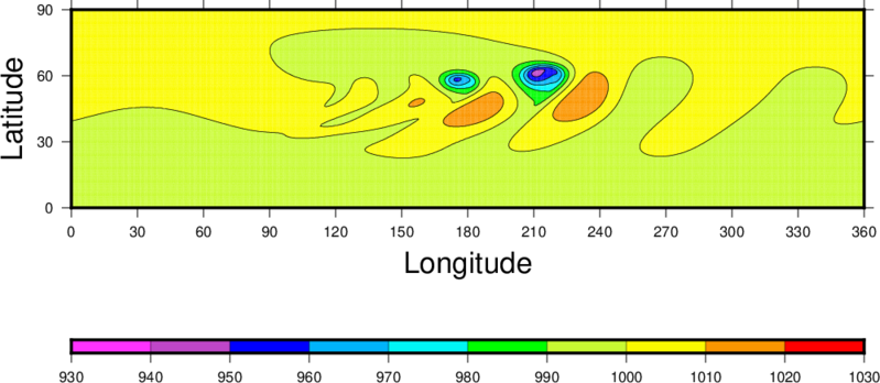
The surface pressure field with the non-hydrostatic module on (again on a 0.7500 x 0.9375 degree lat-lon grid) is shown below. The minimum and maximum surface pressure values at day 9 are 945.296892 and 1018.256570 mb, respectively. Differences with the hydrostatic simulation (less than 1 mb) are, as one should expect at these horizontal resolutions, exceedinly small. 
The same field is shown below but for the hydrostatic simulation on a 1.40625 x 1.875 degree lat-lon grid. Consistent with other studies, the amplification is damped (the minimum and maximum surface pressure values at day 9 are 949.838403 and 1017.841544 mb, respectively) owing to the more coarse horizontal resolution. The non-hydrostatic case is not shown since the impact is even less than for the case on the higher resolution grid. 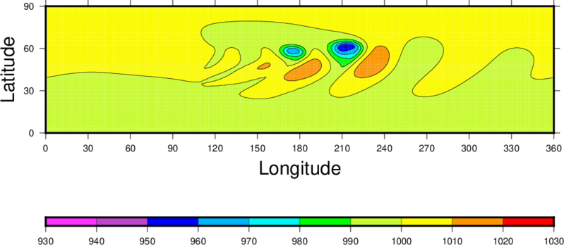
Non-hydrostatic Warm bubble testKilometric scale dry Gaussian initial perterbation
The warm bubble evolution after 540s of integration. The X-axis and Y-axis correspond to distance in km. An animation using ASP for the classic warm bubble test (plotted using standard contour intervals) used for benchmarking non-hydrostatic dynamic cores is shown. The simulation lasts 2500 seconds with a rigid upper lid at about 23.9 km height, uses an initial Gaussian potential temperature perterbation of 6.6 C with calm winds, the upper boundary condition is no flux and w=0, a constant atmospheric potential temperature distribution in both the vertical and the horizontal at 30 C, the pressure at the model top is 50 mb, the horizontal grid spacing is 100 m (20 km length), the domain consists in 200x200 grid cells thus the vertical resolution is also approximately 100m. The bubble is itialized at 2750m above the ground, and extends 2500m in both the horizontal and vertical directions. This case has been widely used (references to be added here) in the atmospheric modeling community for decades. Concerning ASP options, for this case the only diffusion active is 6th order in the z and x-directions. The diffusivity is 0.10 X the maximum value (note, tests have also been done with factors of 0.01, 0.001, 0.0001....: as the factor decreases, more rotars form but solutions become slightly more noisy also as the factor becomes small). All other damping (divergence damping for example, Raleigh sponge layer relaxation or diffusion, etc.) and filtering (other diffusion options) are off. For this simulation, the model is using 5th order horizontal advection and 4th order vertical advection. There is also an animation for the same configuration using continuous contours (more fluid-like) for 2400s of simulation with a rigid top at 175 mb or about 17.5 km. Metric scale dry Gaussian initial perterbation: Robert bubble testThese tests were inspired by the work of Robert et al. (1993) who did dry adiabatic tests using an initial Gaussian temperature perterbation of 0.5 C in a neutral atmosphere, similar to the previous experiments but at a 10 m resolution (with a vertical domain extending up to about 1500 m). The bubble resembles quite closely the bubble they presented after 18 minutes of integration, with slight differences likely arising to differences in numerics (they used a semi-implicit scheme time integration scheme, while ASP uses an explicit scheme with high-order (5th in the horizontal, 4th in the vertical) finite differences. An animation of the bubble using same initial perterbation but at a 5 m resolution, is characterized by more shear-induced rotars. This illustrates the well-known structural-dependence of the convective bubbles on resolution. Finally, an additonal simulation has been done using a WENO 5th order scheme for horizontal advection of u, w, potential temperature and geopotential, and also for the vertical advection of u, w, potential temperature, while geopotential is vertically advected using a 4th order centered scheme. The rigid lid is set at about 1500m, thus the bubble hits the upper boundary and spreads out (the simulation is twice as long as the original one shown by Robert et al.). All explicit numerical diffusion is off for this run. Note that for this simulation, no negative temperature values arise which suggests the other schemes lead to oscillatory behavior thereby enducing negative temperature values. The main bubble structrure is similar, however, wake structures are a bit different. Non-hydrostatic Cold bubble test
The cold bubble evolution after 900s of integration. An animation using ASP for the classic cold bubble test used for benchmarking non-hydrostatic dynamic cores is shown (there is also a corresponding animation over a zoomed-in part of the domain). The simulation lasts 900 seconds, uses an initial potential temperature perterbation of -15 K with calm winds, the upper boundary condition is no flux and w=0, a constant atmospheric potential temperature distribution in both the vertical and the horizontal at 300 K, the pressure at the model top is 50 mb, the horizontal grid spacing is 100 m (40 km length), the domain consists in 400x200 (x,z) grid cells thus the vertical resolution is also approximately 100m. The bubble is itialized at 3000m above the ground, and extends 4000m in the horizontal and 2000m in the vertical directions. This case has been widely used (references to be added here) in the atmospheric modeling community for decades. Concerning ASP options, for this case the only diffusion active is 2nd order in the x and z directions with a constant diffusivity of 75 m2/s: this is used for comparison with other studies. All other damping (divergence damping for example, Raleigh sponge layer relaxation or diffusion, etc.) and filtering (other diffusion options) are off. 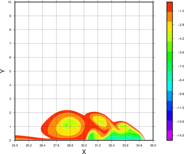
Snapshot of the potential temperature perterbation at 900s using the standard color scale seen in several publications. There is also an animation for the same configuration using continuous contours (more fluid-like). When this cold bubble case was originally defined years ago, 2nd order diffusion was required to maintain numerical stability. However, now improved numerical techniques can permit cold bubble simulations using higher order more-scale selective diffusion. The above simulation has been rerun using 6th in place of 2nd order diffusion with an appropriately scaled diffusivity, which is defined as 75/16 m6/s. The corresponding animation over a zoomed-in part of the domain reveals an additional rotar which was damped out in the baseline benchmark simulation, along with some other interesting features. In addition, the simulation is run 4x longer than the baseline simulation, which permits the density current to hit the lateral rigid boundaries. Note, the model equations are in flux form, so that both the dynamics and horizontal diffusion prescribe zero flux at the lateral boundaries. Also note that in the 3 points closest to each lateral boundary, the order of the horizontal advection and diffusion are reduced to second order schemes. Tests have shown that the domain average potential temperature and the mass are very highly conserved (for example, for these simulations, domain averaged potential temperature is conserved to within 0.0006 K and mass is conserved to within 5x10-11 Pa). This is purely an academic test, but it illustrates the impact of diffusion (perhaps in the future, a similar more modern benchmark can be envisioned). Mountain wave tests using the new non-hydrostaic coreHere are a set of standard mountain wave benchmark tests for a stably stratified atmosphere and constant horizontal flow entering the domain laterally. Mainly the height and slope of the surface topography varies among the tests. NOTE: More information and references will soon be provided. Linear hydrostatic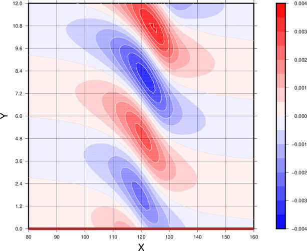
The vertical velocity, w, in m/s. Y corresponds to height (km), and X corresponds to horisontal distance (km). Linear non-hydrostatic
The vertical velocity, w, in m/s. Y corresponds to height (km), and X corresponds to horisontal distance (km). Non-linear non-hydrostatic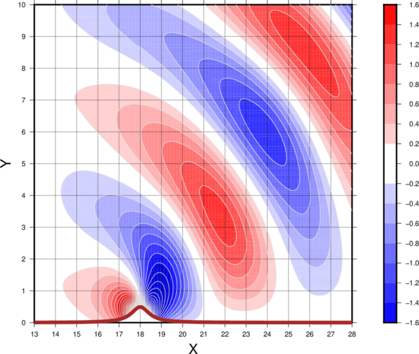
The vertical velocity, w, in m/s. Y corresponds to height (km), and X corresponds to horisontal distance (km). Schaer-type mountain range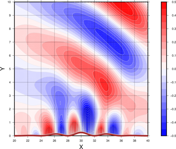
The vertical velocity, w, in m/s. Y corresponds to height (km), and X corresponds to horisontal distance (km). Feel free to send any comments (aaron.a.boone@gmail.com). DisclaimerPlease note that this page has nothing to do with my employer, CNRS, or where I am employed, at the National Center for Meteorological Research (Centre National de Recherches Meteorologiques: CNRM) at Meteo-France. The opinions expressed herein are my own, and are not a reflection of those where I work or of my employer. |